How to Paint a 3-D Brain Volume with a Focused-Ultrasound Spot

Imagine painting the inside of an egg-shaped volume with a brush whose tip is small and elongated, whose paint dries out within a minute, and which you are only allowed to touch the surface with in short bursts. That is roughly the planning problem behind volumetric blood–brain barrier opening with focused ultrasound, and it is the problem my colleagues and I worked on at ICube (Strasbourg) with B. Larrat, F. Nageotte and J. Vappou ^{[1, 2]}.

The barrier, and the spot

The blood–brain barrier (BBB) protects the central nervous system by keeping large molecules out of it. That protection is also why many drugs never reach brain tumors or regions affected by neurodegenerative diseases. Focused ultrasound (FUS) offers a way around it: microbubbles injected into the blood oscillate in the ultrasound focus, and above a threshold the barrier opens locally and reversibly.

The catch is the size of the spot. Clinical FUS devices permeabilize small focal regions. To treat an extended target, the usual approach is to sonicate adjacent points one after another until the region is assumed to be covered. In the words of our paper, this makes the operation "tedious and inaccurate".

Why naive scanning is not enough

A raster scan, sweeping the focus line by line through the target, looks like the obvious fix. Three things work against it.

The paint dries. Microbubble concentration decays exponentially after injection; in our experiments their useful lifespan was about 60 s. A point visited late in a scan receives much less effect than a point visited early, at the same pressure.
The brush is elongated. The focal volume of the transducer is long along the beam axis and narrow across it, so a uniform grid of points does not give a uniform dose.
The scan has to be fast and even at the same time. Spending more time on each point improves coverage but costs time the microbubbles do not have, and over-exposed regions next to under-exposed ones are exactly what a clinician does not want.

Formally, this coverage planning problem is NP-hard. We therefore did not try to solve it in closed form; we built a simulator, defined what "good" means, and let an optimizer search.

The first chart is the simulator equation in miniature. Move the sliders and the predicted intensity saturates as the microbubbles run out; a lower duty cycle scales the effect down.

Explorable model from the simulator equation

I = M\int c(t)\,p\,dt + A

with the calibrated

M = 6.1\times10^{-4}

and

A = 8.1\times10^{-4}

s$^{-1}$. Assumptions (mine):

c(t)=e^{-t/\tau_c}

(the paper states only a ~60 s lifespan), pressure fixed at 0.43 MPa and normalized to 1, a duty cycle treated as an equivalent reduction of sonication time (as in the paper). The absolute exposure scale is indicative; the saturation and the duty-cycle scaling are the point.

A simulator calibrated on a rat

The simulator predicts, for every voxel, how strongly the barrier opens. It integrates the product of microbubble concentration and acoustic pressure over time:

I(X) = M \int c(t)\,p(X,t)\,dt + A

Two constants link this exposure to what an MRI scan actually shows. We obtained them from a rat experiment: two lines sonicated at 0.43 MPa, one with continuous ultrasound and one pulsed at a 10 % duty cycle, imaged with T1-weighted MRI and a gadolinium tracer. Matching the simulated and measured profiles of the pulsed line gave $M = 6.1\times10^{-4}$ s$^{-1}$ and $A = 8.1\times10^{-4}$ s$^{-1}$.

The simulator runs on a GPU at a resolution of 0.1 mm (10³ voxels per mm³) and evaluates one candidate trajectory in 10 to 20 s. That speed is what makes optimization possible at all.

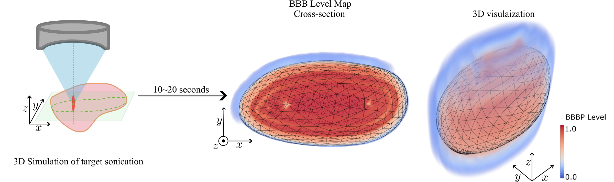A transducer focusing on a target slice, an arrow labeled 10 to 20 seconds, then the simulated permeabilization level map in cross-section and in 3-D over the target mesh. From a candidate trajectory to a 3-D permeabilization map in 10 to 20 s of simulation.

What the optimizer balances

Each candidate trajectory is a stack of layers, and each layer is a spiral. The spiral's loops get closer together as it progresses, so the parts sonicated later, with fewer microbubbles left, receive more overlapping passes. A handful of parameters describe the whole trajectory: the initial loop distance, the rate at which it shrinks, and the velocity profile of the transducer.

The optimizer scores a trajectory with a loss made of three terms, one per objective:

L_G(\Lambda) = f(T) + g(C) + h(H)

Time $T$ , penalized linearly.
Coverage $C$ , rewarded through a sigmoid-shaped term whose best value sits near 90 % rather than 100 %. Chasing the last few voxels usually costs a lot of time and homogeneity for little benefit.
Homogeneity $H$ , the normalized spread of intensity inside the target, penalized so that no region is overdosed while another is missed.

The weights are left to the operator: a clinician can trade time for coverage explicitly instead of implicitly.

To search, we used Hooke–Jeeves pattern search: nudge each parameter, keep the move if the loss drops, shrink the step when nothing helps. It needs no gradient, which matters when every evaluation is a simulation. In practice it converges within about 160 simulation runs, roughly 5 minutes on an average computer, which is compatible with planning before a session.

The interleaving trick

The most useful idea in this work is about timing, not geometry. The transducer is a phased array, so the focus can be moved in two ways: mechanically, by the robot moving the transducer, which is slow; and electronically, by changing the phases of the array elements to shift the focus in depth, without moving anything.

Cavitation-inducing ultrasound is not continuous: it is pulse-width modulated, ON for 1 to 10 % of each period. The rest of the period is idle. We issue the electronic steering command during that OFF time, so that the next pulse lands on another layer. One PWM period can then serve several layers, and each layer still receives the same pulse energy as before. The robot only has to cover the in-plane motion; depth is handled electronically.

Back-of-envelope bound: with a 1-10 % duty cycle, at most $1/d$ equal-dwell layers fit in one period; the slider

u

discounts OFF time lost to refocusing. This is my simplified reading of the mechanism, not a reported result; the measured gain is in the next chart.

What the experiments showed

We tested the optimizer on 512 randomly generated target shapes: 16 sizes from 1.5 to 5.0 mm, 16 aspect ratios from 1.0 to 2.0, and two orientations (0° and 60°). A shape counted as treated if the optimizer found a trajectory with at least 80 % coverage in at most 60 s.

With interleaving and no rotation, every shape up to 4.2 mm was treated; above that size the optimizer failed. The aspect ratio had little influence on that limit.
Switching electronic steering off reduced the maximum treatable volume by about four times.
Orientation helps. Tilting a target so that its long axis comes closer to the beam axis gives electronic steering 1.2× to 2.0× more slices to work with at 60°, and shrinks the footprint the robot has to sweep. For a 4.0 mm target, the loss kept decreasing as the rotation went from 0° to 90°. This suggests that where the transducer is placed around the skull is itself a planning variable.

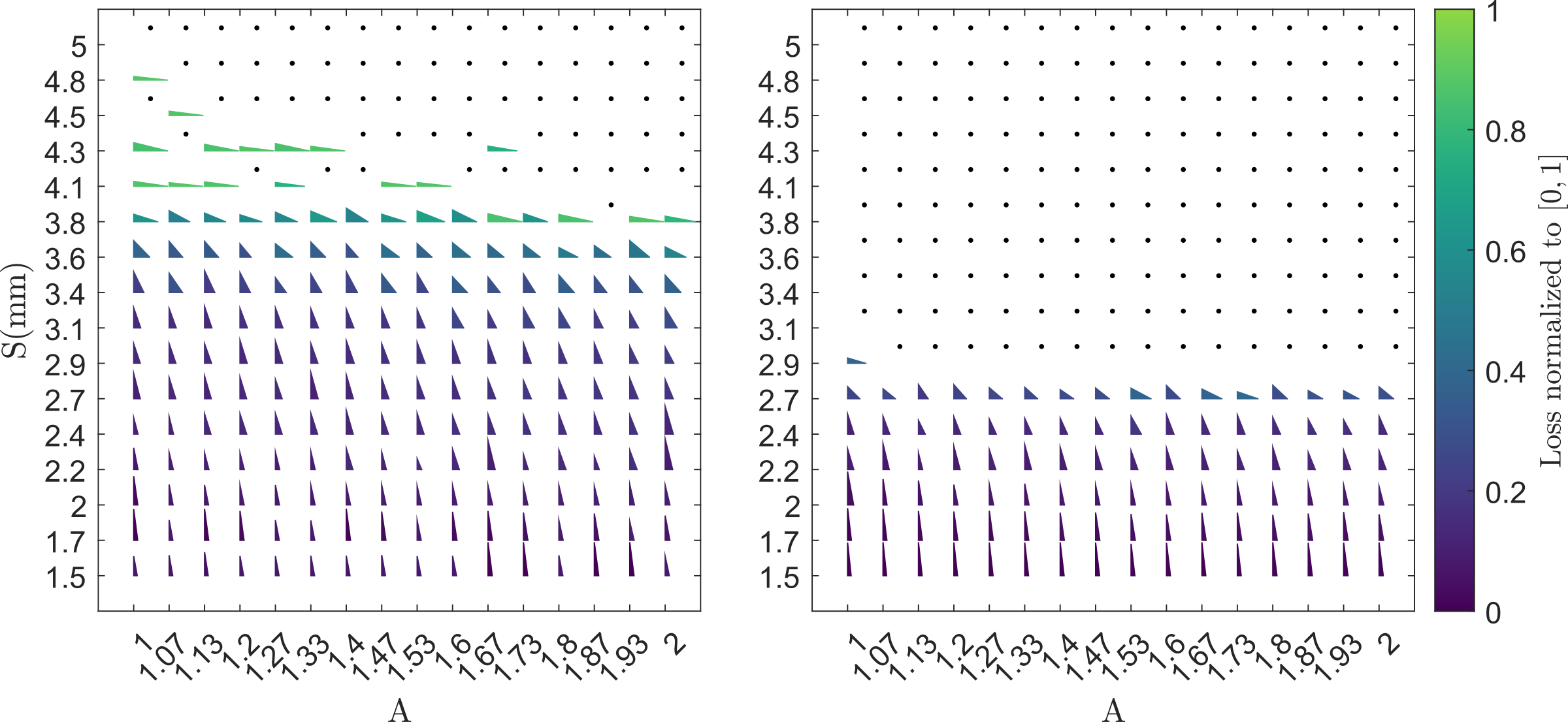Interleaving gives about a 4-fold increase in maximum treatable volume over mechanical steering alone (at least 80 % coverage in under 60 s; 512 random shapes; simulation). Approximate ratio as reported, not absolute volumes. In the same experiment the optimizer reaches sizes up to 4.2 mm at 0 degrees rotation.

Two 16 by 16 result grids over target size and aspect ratio; the left grid, with interleaving, has solved cases at larger sizes than the right grid, mechanical steering only, where black dots mark coverage below 80 %. Interleaved steering (left) against mechanical steering only (right). Triangle height is coverage, width is time, color is the normalized loss; black dots mark coverage below 80 %.

From paper to patent to license

The combination at the heart of this work, mechanical and electronic steering interleaved along a computed trajectory, is protected by patent EP4445859A1 ^[3] (Google Patents, Espacenet). In 2026 it was licensed to Therasonic, a CEA NeuroSpin spin-off. I told that part of the story in a separate post; the technical reference for the optimizer is on its project page.

Limitations

These results are in simulation. The simulator is deliberately simple and empirical, and it was calibrated on two sonicated lines in a single rat, assuming the gadolinium signal is conserved between sonication and imaging. The biophysics of microbubble-mediated opening is still not fully described, so more targeted in vivo experiments are needed to confirm the simulator's form before its predictions can be trusted for patients. What the work does show is that, once a calibrated model exists, planning a volumetric treatment becomes an optimization problem that a computer can solve in minutes, and that using the idle part of each ultrasound pulse is one of the cheapest ways to make the treatable volume larger.

References

Adnan Saood, Florent Nageotte, Benoit Larrat, Jonathan Vappou. Design of Robotic Trajectories for Volumetric Ultrasound-induced Blood-Brain Barrier Permeabilization. International Symposium on Therapeutic Ultrasound (ISTU), Lyon, France, May 2023, 2023.
Adnan Saood, Maciej Bednarczyk, Benoit Larrat, Jonathan Vappou, Florent Nageotte. Implementation of a Volumetric Blood-Brain Barrier Permeabilization Robotic Platform. Computer and Robot-Assisted Surgery (CRAS), Paris, France, September 2023, 2023.
Adnan Saood, Jonathan Vappou, Florent Nageotte, Benoit Larrat. Focused Ultrasound Sonication with Mechanical and Electronic Steering along a Computed Trajectory. 2024.